1. Introduction
A SAR system can be used for the imagery of the stationary and moving targets. In past years, SAR technology was developed for ground moving target indication (GMTI) applications [
1,
2,
3,
4]. In addition to the military applications of the SAR moving target data, there is a utilization for civil projects, such as traffic monitoring and traffic guidance systems.
Since SAR data preserves the phase, it can be used to estimate the parameters of moving targets. If the SAR raw data contain a moving target, the processed SAR has unfocused and/or displaced areas [
5]. To detect moving targets in single-channel SAR data, researchers have proposed many methods based on the spectrum filtering algorithm [
6,
7], shear average algorithm [
8], RDM (reflectivity displacement method) algorithms [
9], time-frequency analysis algorithm [
5,
10], sub-aperture algorithm [
11], keystone transform algorithm [
12], wavelet transform algorithm [
13,
14], and so on. To evaluate the performance of these methods, the researchers need various SAR raw data containing moving targets with different velocities in different directions, clutter model types, different noise models, etc. The cost of the flight tests for the raw data generation is very high and all of these conditions cannot be performed in the flight tests. Simulated SAR raw data are not a substitution for the real SAR data, but it is a complementary tool for the mentioned works.
Up to now, various SAR simulators were implemented. Franceschetti et al. [
15] classified the SAR raw data simulators into two groups: the SAR processing-oriented simulator and the SAR-oriented simulator. The first group uses the reflectivity function for the raw data generation and the latter group takes account system parameters in the simulation process. Each of these groups can be developed in the time or the frequency domain or hybrid time/frequency domain. Allan et al. [
16,
17] presented a time domain SAR signal simulator for fixed and moving targets, as well as clutter, and then developed it in the multichannel SAR system. Geng et al. [
18] proposed a frequency spectrum model for the radar signal to simulate the SAR raw data in the frequency domain (2FD). Dogan et al. [
19] simulated an extended scene and the moving target in the frequency domain separately and then superposed them in the time domain.
The time domain simulator computes the reflection from individual points or facets in the scene and provides a realistic simulation. However, the extended scene simulation is time-consuming. The frequency domain simulation reduces this computational load by some approximations. Hybrid time/frequency domain simulators attempt to decrease these approximations.
In recent years, the reverse of SAR imaging methods has been used to generate SAR raw data. In these methods, first, the SAR image is simulated and then the reverse of an imaging algorithm is applied.
There are several inversion methods for the raw data simulation, such as IOK (inversion of ω–k algorithm [
20,
21]), IPFA (inversion of polar format algorithm [
22]), ICS (inversion of chirp scaling algorithm [
20,
23]), IRD (inverse of range-Doppler algorithm [
24]), and inverse-EETF4 (inverse of extended exact transfer function, 4th-order [
25]). The IOK method has an interpolation step that is not perfectly inverted of the direct method and some errors appear in the final data [
26]. IPFA and IRD methods also contain interpolation processes whose computational load is very high [
26]. In addition, the IRD method has an azimuth frequency dependency problem. The ICS algorithm is faster with respect to the mentioned algorithms because it removed the interpolation step by some approximations in its algorithm, such as ignoring the dependence of modified chirp to the range that causes the range phase error [
27].
In the inverse imaging simulation, we require backscattering of artificial targets and the natural environment. This can be obtain from a focused SAR image or simulated by a reflectivity map.
Speckle and clutter in the SAR data can be a problem in the moving targets parameter estimation [
28]. Chiu et al. [
29] studied the effects of the stationary clutter on the moving target parameters estimation and the results showed errors in target’s azimuth position and radial-velocity estimation. In the moving target detection applications, the background is assumed as clutter (unwanted echoes). The speckle can be directly applied to the image, but it does not consider the filtering properties of the SAR system [
30]. Franceschetti et al. [
31,
32] used a statistical model for considering speckle in the simulation. Some moving target simulation methods neglected the range dependence of the signal model for non-stationary targets [
33] or the azimuth component of the target velocity [
34]. However, in some cases (such as an airborne case), these assumptions might create errors.
In this paper, we propose a method to simulate a scene that has speckle in the frequency domain and moving targets in the time-domain, then integrate these simulations in the time domain. The proposed method presents several advantages. First, it allows simulating speckle at the SAR raw data level. In addition, since all the moving target detection methods, mentioned before, are based on the different Doppler characters of the moving target, the proposed method preserves the phase of the moving targets, which is necessary to evaluate these methods. The rest of the paper is structured as follows:
Section 2 will discuss the methodology of the proposed method,
Section 3 shows the implementation and results, a discussion of the findings is given in
Section 4, and conclusions are drawn in
Section 5.
2. Methodology
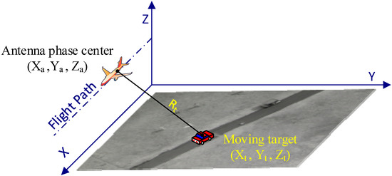
presents the SAR data acquisition geometry relevant to this procedure. This SAR system is a stripmap SAR without any squint (broadside geometry). The system transmits a chirp from the antenna. The antenna phase center is located at (Xa,Ya,Za) and the target coordinate is (Xt,Yt,Zt).
Figure 1. The SAR system geometry.
According to , the flight direction is denoted as the azimuth direction and the line-of-sight as the slant range direction. In all of the figures, the flight direction is taken from top to bottom and the sensor illuminates the scene from the left.
In this paper, we assumed that while the incident angle or incident frequency changed, the SAR system transfer function (STF) is the same for every SAR resolution cell.
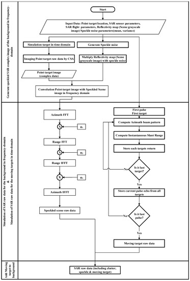
shows the flowchart of the proposed method for the simulation of moving targets in the background. The flowchart can be summarized with the following steps:
-
Generation of the speckled SAR complex image of the background;
-
SAR raw data simulation of the background in the frequency domain;
-
SAR raw data simulation of the moving targets in the time domain; and
-
Integration of two datasets in the time domain.
Figure 2. The SAR raw data simulation flowchart.
2.1. Generation of the Speckled SAR Complex Image of the Background
Noise non-stationary in the scene, and its basic characteristics (variance, probability density function in some limits) vary from one local fragment of an image to another fragment. Noise-like speckle can be viewed as a noise with spatial variation. The probability density function of speckle is related to image forming and the number of looks, and it is not always Gaussian [
35]. After an examination of single-look SAR images by taking fragments (homogeneous regions) of them, Abramov et al. [
36] realized that since both components of complex-valued data of any fragments are Gaussian with approximately the same variance, their amplitude values obey the Rayleigh distribution [
36].
For performing the speckle simulation, first, independent identically-distributed (IID) noise is calculated via:
where μ is the noise mean, σ is the noise standard deviation, and M and N are the dimensions of reflectivity map. The reflectivity map can be considered a grayscale image, such as an aerial optical image in which its grayscale values are normalized and are assumed as the reflectance of the ground targets. Matrix f is convolved with a mean filter to produce the spatially-correlated Gaussian noise. An M×N random matrix is generated based on the Rayleigh distribution and, according to the spatial distribution of Gaussian values, the values of the spatially-correlated Gaussian matrix are replaced by Rayleigh-distributed random values. The mentioned steps guarantee the conditions of the speckle in the real SAR images. Then, the resulting matrix is multiplied on the reflectivity map to generate the speckled reflectivity map.
2.2. SAR Raw Data Simulation of the Background in the Frequency Domain
To simulate the SAR raw data of background, the ICS algorithm is applied. The steps of the ICS algorithm are the reverse of the CSA (chirp scaling algorithm [
23]. Let us assume we have a SAR-focused image or a single look complex (SLC) image as follows [
27,
37]:
where S1(Xa,Ys) is a SAR-focused image, ⊗azimuth is the notation for the convolution along the azimuth direction, ⊗Range is the notation for the convolution along the range direction, L is the synthetic aperture length centered at (Xac,Ya,Za), λ is the wavelength of the transmitted signal, R0 is the broadside range or minimum range to a point target, B is the bandwidth, c is the propagation speed of transmitted signal, Rs is the broadside slant range to scene center, Ys is range position related to scene center, σ(Xa,Ys) is the reflectivity map of targets, fc is the radar center frequency, and A1 is related to the sensor parameters and flight attitude. In the reflectivity map, any target assumed as an ideal point target and its reflectivity is invariant in the SAR sensor frequency.
Indeed, Equation (2) shows the two sinc functions convolved with the reflectivity map in the azimuth and the range direction separately. If we assume that the reflectivity map is just a point (a point target that its backscattering coefficient is 1,
σpoint=1), then we can see that the result of this equation is a point target image (
Spoint target) based on the assumed SAR sensor parameters (Equation (3)). We can replace two sinc functions with
Spoint target as follows:
According to the above part of the flowchart in , the point target was simulated in the time domain with the considered sensor parameters and was processed with CSA to produce Spoint target. Then, S1(Xa,Ys) was produced by convolution of the point target image (Spoint target) with the speckled image of the background. The convolution is done in the frequency domain because of computational time. 2D FFT of Spoint target and the speckled image were calculated and multiplied together. Then, S1(Xa,Ys) was obtained by 2D IFFT of the multiplication result.
The first step on the left side of the middle part of the flowchart in is taking the azimuth FFT of the complex image of the SAR scene (S1(Xa,Ys)). By taking the azimuth FFT, the signal is transformed to the range Doppler domain.
The next step is azimuth decompression. By completing this step, every pixel is expanded as a straight line trajectory. This can be done by multiplying a linear phase term
(φ1) in the range- Doppler domain. This term is a range dependent azimuth matched filter. This filter consists of the azimuth modulation and a phase that will be removed in the chirp scaling process. The phase term
φ1 is as follows:
where bm is a generalized chirp rate, RB is the broadside range, KRc is the transmitted frequency at the radar center frequency scaled by a factor (2c), Ax=1−K2XKRC−−−−−−−√, and KX is the frequency domain component related to Xa.
After range Fourier transformation, the signal is in the 2-D frequency domain. In the next step, the straight line trajectory must change to the echo curved trajectory that is known as range migration. This is achieved by a phase term multiplication. The phase term
(φ2) is a 2-D filter with dependencies on both azimuth and range and it is defined as follows:
where ∆KR is the variation of instantaneous transmitted frequency over the transmitted bandwidth scaled by factor 2c.
The signal is transformed to the range-Doppler domain, by taking the IFFT of the signal. In the range-Doppler domain, each target energy expands along a constant range bin and the range curvature does not depend on the target’s azimuth location [
37].
The next step is the chirp scaling process. In this step, the conjugate of the azimuth-dependent range phase
(φ3) is multiplied with the signal. This phase term caused any range migration curves to have their own curvature because of the SAR data acquisition geometry. The phase term
φ3 is as follows:
Finally, the azimuth IFFT is applied to signal and the SAR raw data results in the time domain.
2.3. SAR Raw Data Simulation of the Moving Targets in the Time Domain
The SAR raw data for the moving targets were simulated in the time domain is based on the Zaharris simulation method [
38]. First, the transmitted signal was assumed as:
where t is the fast time, f0 is the carrier frequency, Kr is the FM (frequency modulation) rate, wr(t)=rect(tTp) is the pulse envelope, and Tp is the chirp pulse duration. After interaction of the signal with the targets, the received signal from the targets in the baseband is converted to:
where η is the slow time, Fm is the normalized reflectivity of point target m, td(t,η)=t−2Rm(t,η)c is the subtraction of pulse travel time for each target from the fast time, Rm (Equation (9)) is the instantaneous slant range of point target m from the antenna phase center, wa(η) (Equation (10)) is the azimuth beam pattern, φ1(t,η) (Equation (11)) and φ2(t,η)(Equation (12)) are the first and the second terms of the phase power series of the received signal (higher terms of phase expansion were assumed to be zero), and nm(t,η) is the additive white Gaussian noise (AWGN).
In Equations (9) and (10), Xc is the center of scene, xm(t) and ym(t) are the instantaneous coordinates of target m, vmyand vmy are the instantaneous velocities of the target m in x– and y-axis, V is the platform speed, ta is the aperture time, La is the antenna length, and λ is the wavelength of signal.
According to the right side of the middle part of the flowchart in , computation of the azimuth beam pattern (Equation (10)), the instantaneous slant range (Equation (9)) and target return (Equation (8)) are repeated for each transmitted pulse and each moving target on the scene.
2.4. Integration of Two Datasets
Finally, the summation of the simulated data of a speckled scene and the simulated data of the moving targets was calculated. The last calculated matrix was the speckled SAR raw data of a scene with the moving targets.
3. Implementation and Results
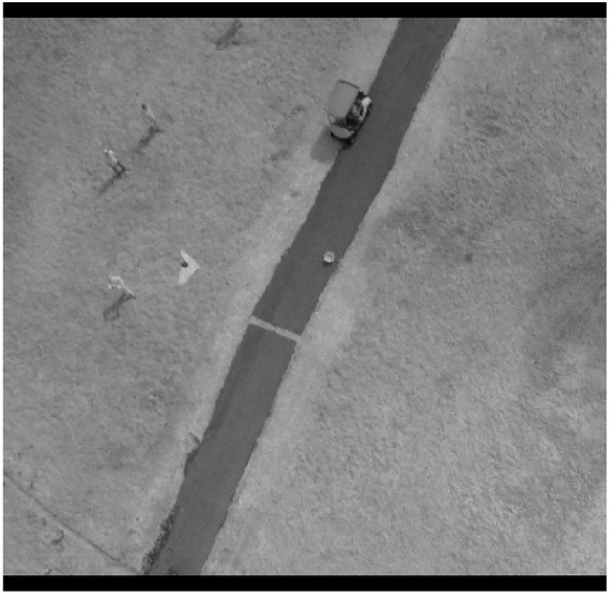
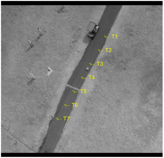
To evaluate the proposed method, a grayscale aerial optical image () was selected as the reflectivity map and the Envisat ASAR sensor selected as the SAR sensor in this research. The sensor’s parameters are described in .
Figure 3. Reflectivity map in grayscale [
39].
Table 1. Parameters of Envisat ASAR sensor.
First, for a given
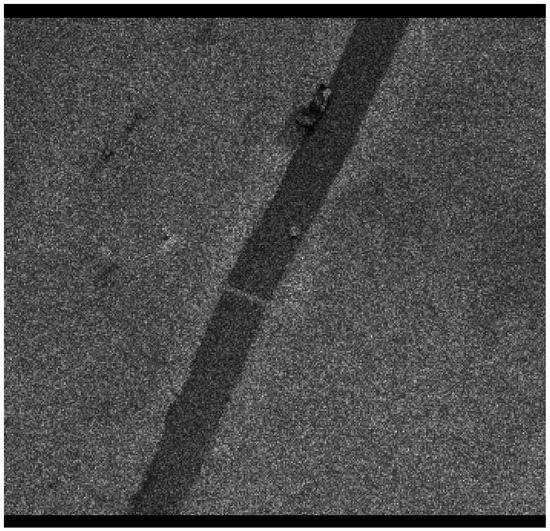
μ=0 and σ2=100, the speckle noise was computed and then was multiplied by the reflectivity map gray values to produce a speckled reflectivity map as . As mentioned in
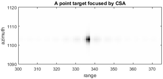
Section 2.2, a single point target was simulated based on the sensor parameters in the time domain simulator and was focused with the CS imaging algorithm (). The resulted SAR single-point image was convolved with the speckled reflectivity map to produce the SAR SLC image as depicted in . Then, the ICS algorithm was applied to the SAR image to generate the SAR raw data of the scene. displays the simulated SAR raw data of the scene. The range-Doppler algorithm (RDA) [
40] and CSA were implemented for evaluating the resulting data.
Figure 4. The reflectivity map with speckle (μ=0 and σ2=100).
Figure 5. Simulated point target (time domain).
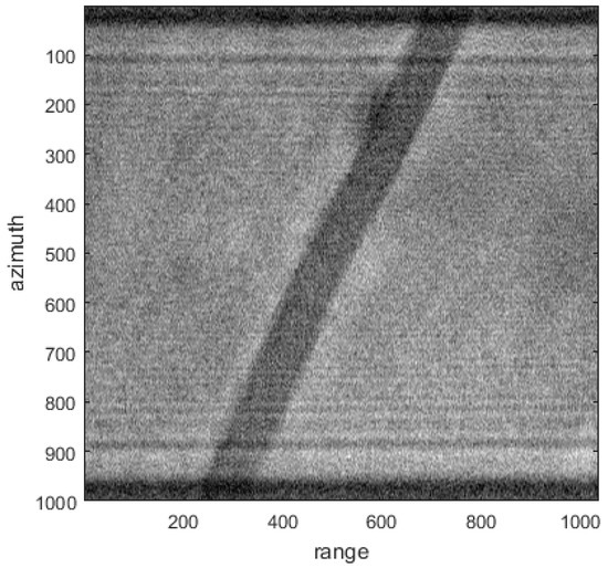
Figure 7. SAR simulated raw data of the scene without moving targets.
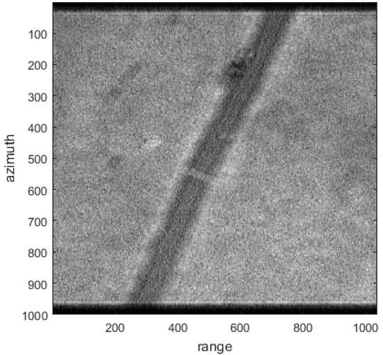
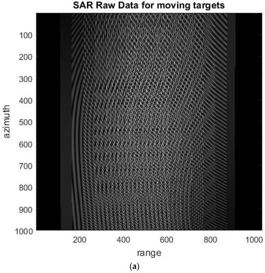
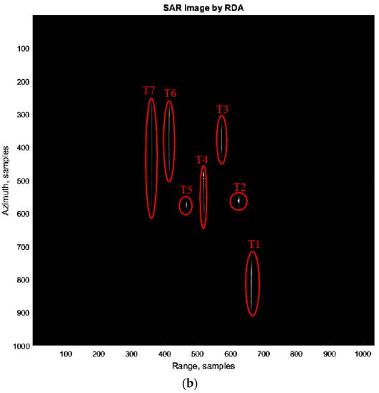
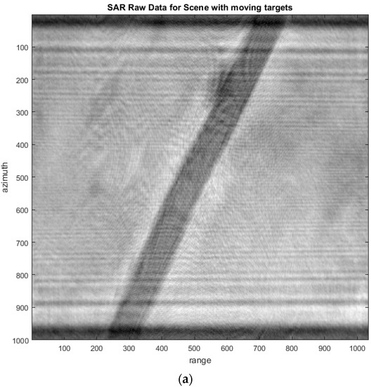
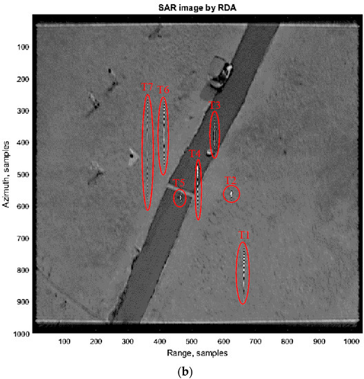
The next step is the simulation of the moving targets. The moving targets were simulated in the time domain. The targets were assumed as the point targets with non-fluctuating RCS. They had a constant velocity or a constant acceleration in a constant direction. They were positioned on the reflectivity map (scene) in different directions, with different velocities and accelerations and their echoes were simulated in the time domain based on Envisat ASAR sensor parameters (). Seven different targets were considered. and show these moving target parameters and their location on the reflectivity map, respectively. a shows the generated SAR raw data for the moving targets in the time domain that are focused by the RDA, as shown in b. b shows the smear and displacement of targets because of their velocities and accelerations. According to , T2 has the range velocity and its location displaced in b. T3 and T4 have the cross-range movements and their images smeared in b. The images of T1, T6, and T7 are not only displaced because of the range velocity, but also smeared because of their cross-range velocity or range/cross-range accelerations. Finally, superimposition of the simulated SAR raw data of the moving targets and the simulated SAR raw data of the scene was computed to produce the SAR raw data of the scene containing the moving target. shows this SAR raw data and its focused image.
Figure 8. Moving target positions in the scene.
Figure 9. (a) The SAR raw data of moving targets (simulated in the time domain) and (b) its focused image.
Figure 10. (a) The SAR raw data of the scene including moving targets and (b) its focused image.
Table 2. Moving target parameter variations in the generated SAR images.
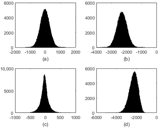
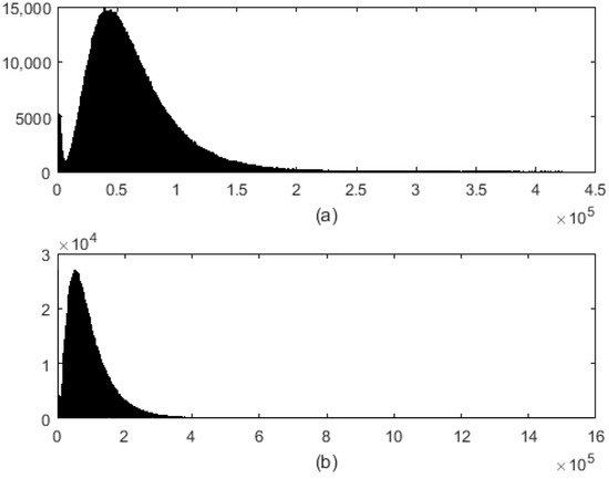
To evaluate the proposed method, the ICS results from the SAR raw data () focused by CSA and RDA. These two images are compared with the reflectivity map. To evaluate the accuracy of the simulated speckle in the images, the histogram of the real and imaginary parts of a homogeneous area of the SAR images (before and after the simulation) were computed. illustrates the Gaussian behavior of this phenomenon. The top figures (the histogram of real and imaginary parts of the SAR image before the simulation) and bottom figures (the histogram of real and imaginary parts of the SAR image after the simulation) have a Gaussian shape and only their variances are different. Additionally, the local variance for each 8 × 8 pixel block of the absolute SAR images was computed. shows that the local variance of the absolute images before and after the simulation has the Rayleigh distribution behavior.
Figure 11. Histograms of the real (a) and imaginary (b) parts of the SAR image (before simulation); and histograms of the real (c) and imaginary (d) parts of the SAR image (after simulation).
Figure 12. The local absolute variance of SAR images (a) before the simulation and (b) after the simulation.
To assess the stability of the spatial changes of the SAR images before and after the simulation, the parameter r was calculated for SAR images via [
41]:
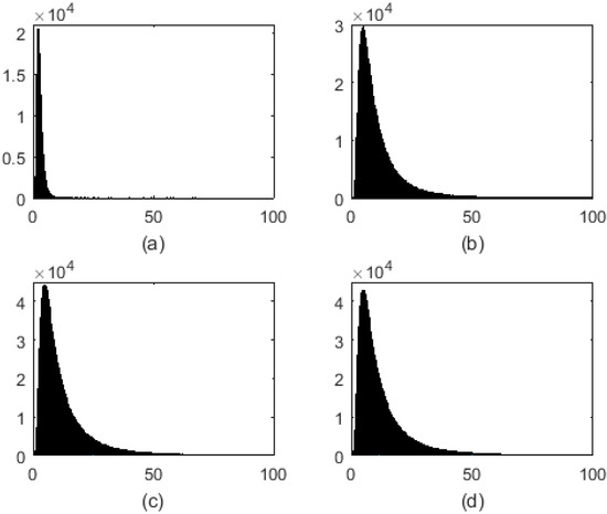
where l and m are the coordinates of 8 × 8 block corner, Iij is the value of pixel (i, j) of the block, is the average value of the block and Dlmqs is an array of DCT coefficients of the block except corner element. In Equation (13), the ratio of two estimations of variance is computed. These two estimations are local variances in the spatial domain and the DCT domain. shows this parameter histogram for different cases.
Figure 13. The histogram of parameter r for (a) the reflectivity map; (b) the absolute SAR image before simulation; (c) the absolute SAR image produced by CSA after simulation; and (d) the absolute SAR image produced by RDA after simulation, respectively.
To analyze the ICS procedure, the correlation coefficients between the SAR images before and after the simulation (without moving targets) were calculated. Based on the SAR image formation method for the simulated SAR raw data, the correlation coefficients for the CSA method and the RDA method were 0.9819 and 0.9719, respectively. This process was repeated for various reflectivity maps and their correlation coefficients between their two SAR images are about 0.95. These coefficients show a reliable relationship between SAR images before and after the simulation.
For locating moving targets, a moving target detection method was developed based on [
42] to test the quality of the moving targets after integrating with the background, the process of which is as follows:
-
Select an image;
-
Compute the azimuth FFT of the image;
-
Separate the positive Doppler data and the negative Doppler data with appropriate band-pass filters;
-
Compute the azimuth IFFT of two sub-data generated in the previous step to produce two symmetric sub-image;
-
Compute the intensity differences of these two sub-images; and
-
Use a threshold to detect the moving target or targets.
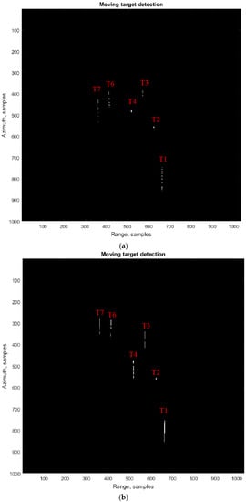
The results of the implementation of this algorithm are presented in a,b for images of moving targets with abackground and without a background, respectively. Some targets in a were partially detected because of background changes along the smeared target.
Figure 14. Results of moving target detection algorithm in SAR images of (a) moving targets with a background and (b) moving targets without a background.
4. Discussion
In this study, we proposed a method to simulate the SAR raw data in the hybrid domain. However, the phase information remains intact, which can be used to estimate moving target parameters. Additionally, the speckle was included within the SAR raw data. Thus, it is possible to evaluate how this problem is handled by moving target detection algorithms.
Both time- and frequency-domain simulators can simulate large backgrounds. According to the time domain algorithm (), there are two loops that must be repeated for each target in the scene and each transmitted pulse. Assuming a scene comprised of M by N pixels in the range and azimuth directions, respectively, we have M × N scatterers. Transmitted pulses consist of nt and na pixels in the time and azimuth directions, respectively, so we have a computational complexity of nt × na per scatterer, and the total number of multiplications is given by M × N × nt × na for the time-domain simulation. However, a frequency domain method, like the ICS algorithm, obtains the raw signal from the image space to the signal space. According to the ICS algorithm (), the number of computations to produce a SAR SLC image from the reflectivity map is 2 × M × N × log2 (M × N) + M × N and the other steps take 4 × M × N × log2 (M) + 3 × M × N computations. By comparing the number of computations, the ICS algorithm is very fast with respect to the time domain simulation. Some researchers simulated moving targets and the background in the time domain. We simulate static and moving targets separately in the proposed method, so there is no computational load problem with large backgrounds (static targets) that were simulated in the frequency domain, and we have a few moving targets (with respect to the scene pixels) that were simulated in the time domain. The problem of the ICS algorithm used in the proposed method is the fact that it cannot consider the precise system transfer function [
16]. Since the purpose of this method is to produce raw SAR data for evaluating moving target detection algorithms, it did not matter. however, an accurate model is necessary for terrestrial remote sensing applications.
In research studies of the simulation of the moving targets in the frequency domain, only a few special cases are considered, such as a fixed target velocity [
19]. Additionally, they have a phase error because of the approximation in their algorithms [
27]. In the proposed method, moving targets are simulated in the time domain for the preservation of the phase. The phase is responsible for the signal structure and the phase error causes displacement in target locations. illustrates that there is no difference in moving target locations between the proposed method and time domain simulation.
For performing the speckle simulation, the speckle properties of Sthe AR raw data simulated by the proposed method (, and ) were examined. The result showed similar speckle properties of the real SAR data as in [
36] and the simulation is also faster than the time domain methods.
5. Conclusions
For the importance of the moving target detection in clutter, a new method to simulate moving targets on the speckled scene is proposed. The proposed method consists of three main parts. The first part is generating the speckled SAR complex image of the background. The histogram of real and imaginary parts of a homogeneous area from the speckled SAR images (before and after the simulation) showed the Gaussian behavior of the speckle and the local absolute variance of the images (before and after the simulation) showed the Rayleigh distribution behavior. The second part is the SAR raw data simulation of the background. The SAR simulation of the distributed target in the time domain has a computational load. Using the frequency domain simulation, like the ICS algorithm, is so fast that we can simulate a large scene (e.g., 1000 × 1000) in a few seconds.
For various reflectivity maps, the second part was repeated and after focusing the SAR raw data (by RDA and CSA), their correlation coefficients between their two SAR images (before and after the simulation) were about 0.95. By considering the speckle in the reflectivity map, the first and the second part were integrated together and we could produce the SAR raw data with spatially-correlated speckle. The third part is the SAR raw data simulation for the moving targets in the time domain. The resulting simulation in the third part was integrated with previous parts. The results showed the efficiency of the calculations for the proposed technique. There are no limitations for direction, velocity, and acceleration in the proposed method, and the results show that there is no change in the targets’ locations after detection in the two simulated datasets (one simulated by the proposed method and the other one simulated in the time domain). Moreover, the quality assessment of the results showed that the generated raw data could meet the radiometric and geometric requirements. Geometric requirements mean that the location of the moving targets in the scene must be the same in the time domain simulation and the proposed method. Radiometric requirements mean that the gray value of the targets of the scene (the reflectivity map), as well as the noise behavior, must bethe same before and after the simulation. Additionally, various simulations showed that the targets could still be identified by changing the contribution of the background’s data and moving targets’ data.
Our simulation capabilities, in comparison with other moving target simulations, were considering a background scene of any size, generating speckled raw data and preserving the phase for moving target parameters estimation. In future works, one can directly simulate the SAR image based on various algorithms.